
Pre-note If you are an early stage or aspiring data analyst, data scientist, or just love working with numbers clustering is a fantastic topic to start with. In fact, I actively steer early career and junior data scientist toward this topic early on in their training and continued professional development cycle.
Learning how to apply and perform accurate clustering analysis takes you though many of the core principles of data analysis, mathematics, machine learning, and computational science. From learning about data types and geometry, confusion matrix, to applying iterative aglorithms and efficient computation on big data. These foundational concepts crop up in most other areas of data science and machine learning. For instance, cluster distance matrices underpin and, mathematically, are near identical to graph data structures used in deep learning graph neural networks at the cutting edge of artificial intelligence research. So if you are just starting then don’t be put of and read on regardless of your level. We all have to start somewhere and this is a very good place!
Cluster analysis is the task of grouping objects within a population in such a way that objects in the same group or cluster are more similar to one another than to those in other clusters. Clustering is a form of unsupervised learning as the number, size and distribution of clusters is unknown a priori. Clustering can be applied to a variety of different problems and domains including: customer segmentation for retail sales and marketing, identifying higher or lower risk groups within insurance portfolios, to finding storm systems on Jupyter, and even identifying galaxies far far away.
Many real-world datasets include combinations of numerical, ordinal (e.g. small, medium, large), and nominal (e.g. France, China, India) data features. However, many popular clustering algorithms and tutorials such as K-means are suitable for numerical data types only. This article is written on the assumption that these methods are familiar - but otherwise Sklearn provides an excellent review of these methods here for a quick refresher.
This article seeks to provide a review of methods and a practical application for clustering a dataset with mixed datatypes.
To evaluate methods to cluster datasets containing a variety of datatypes.
The California auto-insurance claims dataset contains 8631 observations with two dependent predictor variables Claim Occured and Claim Amount, and 23 independent predictor variables. The data dictionary describe each variable including:
OLDCLAIM = sum $ of claims in past 5 years
1 2 3 4 5 6 7 8 9 10 11 12 13
# load data DATA_PATH = os.path.join(os.getcwd(),'../_data') raw = pd.read_csv(os.path.join(DATA_PATH,'car_insurance_claim.csv'),low_memory=False,) # convert numerical-object to numericals for col in ['INCOME','HOME_VAL','BLUEBOOK','OLDCLAIM', 'CLM_AMT',]: raw[col] = raw[col].replace('[^.0-9]', '', regex=True,).astype(float).fillna(0.0) # clean textual classes for col in raw.select_dtypes(include='object').columns: raw[col] = raw[col].str.upper().replace('Z_','',regex=True).replace('[^A-Z]','',regex=True) data_types = f:t for f,t in zip(raw.columns,raw.dtypes)>
Apply processing to correct and handle erroneous values, and rename fields and values to make the data easier to work with. Including:
1 2 3 4 5 6 7 8 9 10 11 12 13 14 15 16 17 18 19 20 21 22 23 24 25 26 27 28 29 30 31 32 33 34 35 36
# copy df df = raw.copy() # drop ID and Birth df.drop(labels=['ID','BIRTH'],axis=1,inplace=True) # remove all nan values df['OCCUPATION'].fillna('OTHER',inplace=True) for col in ['AGE','YOJ','CAR_AGE']: df[col].fillna(df[col].mean(),inplace=True) if df.isnull().sum().sum() == 0: print('No NaNs') data_meta = pd.DataFrame(df.nunique(),columns=['num'],index=None).sort_values('num').reset_index() data_meta.columns = ['name','num'] data_meta['type'] = 'numerical' # exclude known numericals data_meta.loc[(data_meta['num']15) & (~data_meta['name'].isin(['MVR_PTS','CLM_FREQ','CLAIM_FLAG'])),'type']='categorical' data_meta.loc[data_meta['name'].isin(['CLM_FREQ','CLAIM_FLAG']),'type']='claim' categorical_features = list(data_meta.loc[data_meta['type']=='categorical','name']) numerical_features = list(data_meta.loc[data_meta['type']=='numerical','name']) # shorten names df['URBANICITY'] = df['URBANICITY'].map('HIGHLYURBANURBAN':'URBAN', 'HIGHLYRURALRURAL':'RURAL'>) df['EDUCATION'] = df['EDUCATION'].map('HIGHSCHOOL':'HSCL', 'BACHELORS':'BSC', 'MASTERS':'MSC', 'PHD':'PHD'>) df['CAR_TYPE'] = df['CAR_TYPE'].map('MINIVAN':'MVAN', 'VAN':'VAN', 'SUV':'SUV', 'SPORTSCAR':'SPRT', 'PANELTRUCK':'PTRK', 'PICKUP':'PKUP'>)
No NaNs
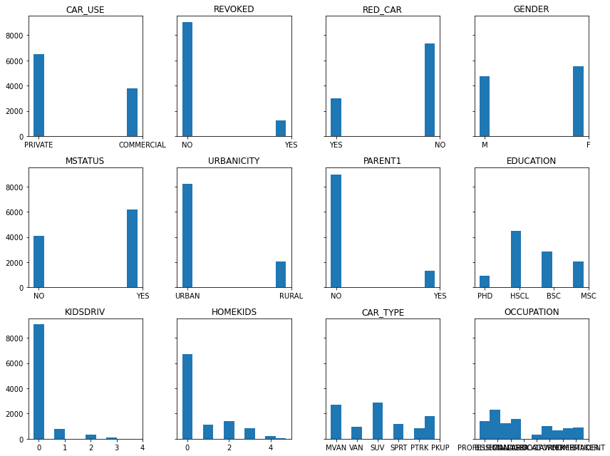
Categorical feature histograms
Shown below are the histogram of each categorical feature. This illustrates both the number and frequency of each category in the dataset.
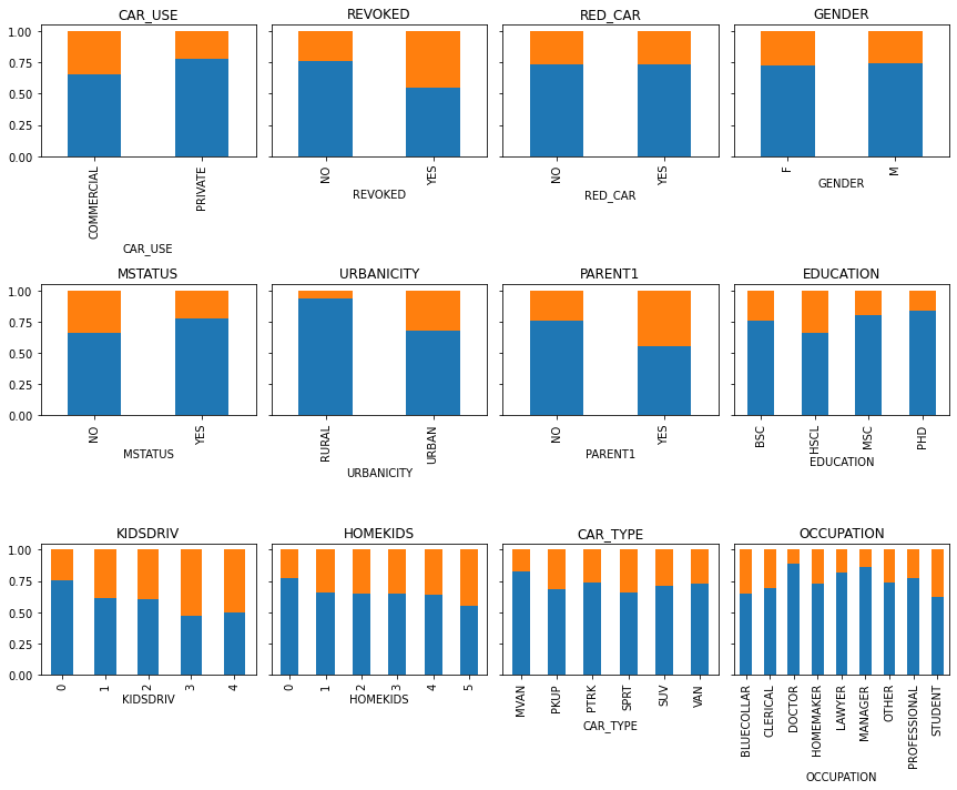
How are claims distributed amongst the categorical features?
As above, the bar plots again illustrate each categorical feature and value, but now also show how the proportion of claims is distributed to each categorical value. For example, Commericial CAR_USE has a relatively higher proportion of claims than Private car use.
Recall that each clustering algorithm is an attempt to create natural groupings of the data. At a high-level, clustering algorithms acheive this using a measure of similarity or distance between each pair of data points, between groups and partitions of points, or between points and groups to a representative central point (i.e. centroid). So while the actual algorithm impementations to achive this vary, in essence they are based on this simple principle of distance.This is illustrated quite nicely in illustration below that shows a data set with 3 clusters, and iterative cluster partitioning a-f by updating the centroid points (Chen 2018). Here the clusters are formed by measuring the distance between each data point (solid fill) and a representative centoid point (hollow fill).

Because clustering algorithms utilise this concept of distance both it is crucial to consider both:
Below are some of the common distance measures used for clustering. Computational efficiency is important here as each data feature introduces an additional dimension.For clustering, by definition, we often have multiple features to make sense of and therefore the efficiency of the calculation in high dimensional space is crucial.
Euclidean distance is the absolute numerical difference of their location in Euclidean space. Distances can be 0 or take on any positive real number. It is given by the root sum-of-squares of differences between each pair (p,q) of points. And we can see that for high dimensions we simply add the distance.
Manhattan distance is again the sum of the absolute numerical difference between two points in space, but using cartesian coordinates. Whilst Euclidean distance is the straight-line “as the crow flies” with Pythagoras theorem, Manhattan takes distance as the sum of the line vectors (p,q).
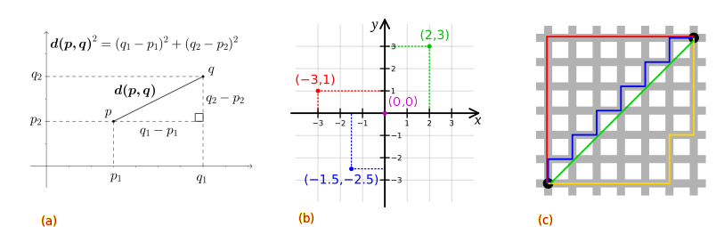
This image illustrates examples for: a) Euclidean space distance, b) Manhattan distance in cartesian coordinate space, and c) both with the green line showing a Euclidean path, while the blue, red, and yellow lines take a cartesian path with Manhattan distance. This illustrates how clustering results may be influenced by distance measures applied and depending on whether the data features are real and numeric or discrete ordinal and categorical values. In addition, perhaps this also illustrates to you how and why geometry and distance are important in other domains such as shortest path problems.
There are many distance metrics (e.g. see these slides). Minkowski distance for example, is a generalization of both the Euclidean distance and the Manhattan distance. Scipy has a convenient pair distance pdist() function that applies many of the most common measures.
Example:
from scipy.spatial.distance import pdist pdist(df,metric='minkowski')
There are also hybrid distance measures. In our case study, and topic of this article, the data contains a mixture of features with different data types and this requires such a measure.
Gower (1971) distance is a hybrid measure that handles both continuous and categorical data.
The Gower distance of a pair of points $G(p,q)$ then is:
where $S_$ is either the Manhattan or DICE value for feature $k$, and $W_$ is either 1 or 0 if $k$ feature is valid. Its the sum of feature scores divided by the sum of feature weights.
With this improved understanding of the clustering distance measures it is now clear that the scale of our data features is equally important. For example, imagine we were clustering cars by their performance and weight characteristics.
The feature distances between Car A and B are 2.0 seconds and 2000 KG. Thus our 2000 unit distance for mass is orders of magnitude higher than 2.0 seconds for 0-60 mph. Clustering data in this form would yield results bias toward high range features (see more examples in these StackOverflow answers 1,2,3). When using any algorithm that computes distance or assumes normally distributed data, scale your features 4.
For datasets with mixed data types consider you have scaled all features to between 0-1. This will ensure distance measures are applied uniformly to each feature. The numerical features will have distances with min-max 0-1 and real numbers between e.g. 0.1,0.2,0.5,…0.99. Whereas the distances for categorical features be values of either 0 or 1. As for mass KG in the car example above, this could still lead to a bias in the formation of clusters toward categorical feature groups as their distances are always either the min-max value of 0 or 1.
Selecting the appropriate transformations and scaling to apply is part science and part art. There are often several strategies that may suit and must be applied and evaluated in relation to the context of challenge at hand, the data and its domain. Crucially, whatever strategy is adopted, all features in the final dataset that is used for clustering data must be on the same scale for each feature to be treated equally by the distance metrics.
Different data types and how to handle them
Here are two excellent articles and figures that delve deeper on (left) data-types and (right) encoding techniques.
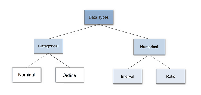

In summary, these are:
Numerical features: continuous and interval features such as mass, age, speed, luminosity, friction.
Nominal Categorical features: Unordered nominal or binary symmetric values where outcomes are of equal importance (e.g. Male or Female).
Ordinal Categorical features: Ordered ordinal or binary asymmetric values, where outcomes are not of equal importance.
By far ordinal data is the most challenging to handle. There are many arguments between mathematical purists, statisticians and other data practitioners on wether to treat ordinal data as qualitatively or quantitatively (see here).
There are also considerations for the clustering algorithm that is applied. These will be introduced and discussed on application to the case study dataset in the results section.
Scaling numerical features
Below, both Standard and MinMax scaling is applied to show how the data is transformed. The MinMax scaled data is used going forward.
from sklearn.preprocessing import scale,RobustScaler,StandardScaler, MinMaxScaler